However I when thinking graphically I think that it is possible to approximate these nonlinear functions using lots of linear ( scaled and shifted) linear lines and I do not understand why this is incorrect.
It's not generally incorrect, but what you are describing there is not a single function but a piecewise function. For example:
$
f(x) = \left\{
\begin{array}{ll}
0.1 x & \quad 0 \leq x < 0.1 \\
0.2 x & \quad 0.1 \leq x < 0.2\\
0.3 x & \quad ...
\end{array}
\right.
$
This composition is non-linear, because the input space gets transformed differently depending on $x$ (because each subfunction in the example above has a different slope). There are methods to optimize such a function as well, e.g. piecewise linear regression.
An MLP without non-linearities is not a piecewise function, but a function composition:
$(f \circ g)(x) = f(g(x))$,
where $g$ and $f$ are two consecutive dense layers.
The difference is that if both functions $g$ and $f$ are linear, then $f \circ g$ is linear. This holds for any configuration of model parameters. Therefore, the model transforms any given input space $X$ into some output space $W$, where straight lines in the input space remain straight in the output space and can thus never model something non-linear.
In case, if it is possible to approximate any function using Relu activation function ( which is linear on first quadrant) , why it is not possible to approximate with a function completely linear ?
As soon as you introduce any non-linearity, the system becomes much more expressive, because each neuron now models a non-linear function. Combining the neurons (as done by a subsequent layer) can learn combinations of these non-linear functions.
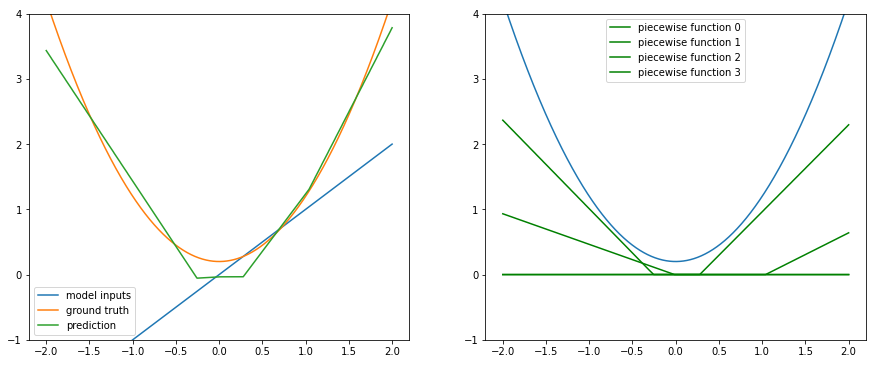
And this is where the two worlds collide: If you take a ReLU activation, it allows the model to actually learn something like a piecewise linear function, because of the combinations of several linear functions with different slopes that are $< 0$ only for certain input ranges. Here is a simple example of that:
import numpy as np
import tensorflow as tf
import matplotlib.pyplot as plt

tf.random.set_seed(4)
np.random.seed(4)

# create a dataset
xs = np.linspace(-2, 2, 1000)
ys = xs**2 + 0.2

# create a model
m = tf.keras.Sequential([
    tf.keras.layers.Dense(4, activation='relu'),
    tf.keras.layers.Dense(1),
])

# train the model
m.compile(optimizer='adam', loss=tf.keras.losses.MAE)
m.fit(xs[:,np.newaxis], ys[:,np.newaxis], batch_size=8, epochs=20, verbose=None)

# plot the results
fig, ax = plt.subplots(1, 2, figsize=(15, 6))

ax[0].plot(xs, xs, label='model inputs')
ax[0].plot(xs, ys, label='ground truth')
ax[0].plot(xs, m(xs)[:,0], label='prediction')
ax[1].plot(xs, ys)

for n in range(m.layers[0].units):
    neuron_act = m.layers[0](xs[:,np.newaxis])[:,n]
    ax[1].plot(xs, neuron_act, color='g', label='piecewise function %d' % n)

ax[0].legend()
ax[1].legend()
ax[0].set_ylim((-1, 4))
ax[1].set_ylim((-1, 4))

The left image shows what the model has learned (green line), the right side shows the functions of the individual neurons. The more neurons you add to that first relu-layer, the better the approximation of the ground truth will be.

