How do I combine two electromagnetic readings to predict the position of a sensor?

Question

I have an electromagnetic sensor and electromagnetic field emitter. The sensor will read power from the emitter. I want to predict the position of the sensor using the reading.

Let me simplify the problem, suppose the sensor and the emitter are in 1 dimension world where there are only position X (not X,Y,Z) and the emitter emits power as a function of distance squared.

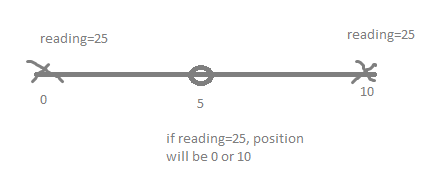
From the painted image below, you will see that the emitter is drawn as a circle and the sensor is drawn as a cross.

E.g. if the sensor is 5 meter away from the emitter, the reading you get on the sensor will be 5^2 = 25. So the correct position will be either 0 or 10, because the emitter is at position 5.

So, with one emitter, I cannot know the exact position of the sensor. I only know that there are 50% chance it's at 0, and 50% chance it's at 10.

So if I have two emitters like the following image:

I will get two readings. And I can know exactly where the sensor is. If the reading is 25 and 16, I know the sensor is at 10.

So from this fact, I want to use 2 emitters to locate the sensor.

Now that I've explained you the situation, my problems are like this:

1. The emitter has a more complicated function of the distance. It's not just distance squared. And it also have noise. so I'm trying to model it using machine learning.

2. Some of the areas, the emitter don't work so well. E.g. if you are between 3 to 4 meters away, the emitter will always give you a fixed reading of 9 instead of going from 9 to 16.

3. When I train the machine learning model with 2 inputs, the prediction is very accurate. E.g. if the input is 25,36 and the output will be position 0. But it means that after training, I cannot move the emitters at all. If I move one of the emitters to be further apart, the prediction will be broken immediately because the reading will be something like 25,49 when the right emitter moves to the right 1 meter. And the prediction can be anything because the model has not seen this input pair before. And I cannot afford to train the model on all possible distance of the 2 emitters.

4. The emitters can be slightly not identical. The difference will be on the scale. E.g. one of the emitters can be giving 10% bigger reading. But you can ignore this problem for now.

My question is How do I make the model work when the emitters are allowed to move? Give me some ideas.

Some of my ideas:

1. I think that I have to figure out the position of both emitters relative to each other dynamically. But after knowing the position of both emitters, how do I tell that to the model?
2. I have tried training each emitter separately instead of pairing them as input. But that means there are many positions that cause conflict like when you get reading=25, the model will predict the average of 0 and 10 because both are valid position of reading=25. You might suggest training to predict distance instead of position, that's possible if there is no problem number 2. But because there is problem number 2, the prediction between 3 to 4 meters away will be wrong. The model will get input as 9, and the output will be the average distance 3.5 meters or somewhere between 3 to 4 meters.
3. Use the model to predict position probability density function instead of predicting the position. E.g. when the reading is 9, the model should predict a uniform density function from 3 to 4 meters. And then you can combine the 2 density functions from the 2 readings somehow. But I think it's not going to be that accurate compared to modeling 2 emitters together because the density function can be quite complicated. We cannot assume normal distribution or even uniform distribution.
4. Use some kind of optimizer to predict the position separately for each emitter based on the assumption that both predictions must be the same. If the predictions are not the same, the optimizer must try to move the predictions so that they are exactly at the same point. Maybe reinforcement learning where the actions are "move left", "move right", etc.

I told you my ideas so that it might evoke some ideas in you. Because this is already my best but it's not solving the issue elegantly yet.

So ideally, I would want the end-to-end model that are fed 2 readings, and give me position even when the emitters are moved. How would I go about that?

PS. The emitters are only allowed to move before usage. During usage or prediction, the model can assume that the emitter will not be moved anymore. This allows you to have time to run emitters position calibration algorithm before usage. Maybe this will be a helpful thing for you to know.

Answer 1

Position Detection

In a traditional data acquisition and control scenario, with some assumptions, the relation between sensors signals $s_i$, emitters drive $\epsilon_j$, distances $x_{ij}$, and calibration factors is modelled as follows.

$$ \forall \, (i, j) \text{,} \quad \frac {s_i} {v_i} = \frac {\epsilon_j} {v_j \, x_{ij}^2} $$

The assumptions include these.

• Linear acquisition of magnetic flux signal strength
• Linear control of magnetic flux signal strength
• Independent readings either by sequential reading or by use of two distinct emitter frequencies
• Dismissal of relativistic phenomena
• Single point emission
• Single point detection

It is correct that, with only a single emitter, position of the sensor cannot be accurately determined because the direction from which the signal originates cannot be disambiguated. Two emitters are necessary for reliability. In two dimensional space, three are necessary, thus the term triangulation. In three dimensional space, four are necessary.

Less Known Function with Motion and Noise

The more complicated function of distance was not specified, whether the sample rate is tightly controlled is not indicated, and the nature and magnitude of the noise relative to the signal was not provided. It also appears there is a low digital accuracy in the readings.

To model these contingencies, for motion, $j$ shall be the sample index, and $i$ remains the detector number. The data acquisition vector is now a tuple of the reading $r_{ij}$ and time $t_j$. The function $f$ may differ from the inverse squared function due to flux conduction curvature, non-point emission and detection, and other secondary effects. The combination of this function and noise $n$, a function of sample time, $s_j$, is made discrete, according to the question, rounding or truncating to the nearest integer (indicated by $\mathcal{I}$).

$$ \forall \, (i, j) \text{,} \quad (r_{ij}, \; t_j) = \bigg(\mathcal{I}\big(f(\epsilon_j, x_{ij}) + n(s_j)\big), \; s_j\bigg) $$

There are other benefits to the additional emitter than disambiguation of direction. The impact of noise is reduced as redundancy is added, and there is the calibration issue.

Calibration

High volume, low cost, electronic parts are not usually calibrated in the factory. Even when they are, the calibration cannot be trusted. Even if calibrated in the factory and then in the lab, the phenomenon of temperature and pressure drift complicates acquisition for passive emitters and transducers. Carefully designed instrumentation and measurement strategy can compensate for component behavioral variance, and redundant emitters and detectors can be used in such designs.

Assuming accuracy above that of a mass produced part is required, the calibration voltages $v_i$ and $v_j$ must be determined simultaneously and be consistently either relative to magnetic flux levels at some point or to each other. If the environment cannot be controlled, re-calibration may be periodically necessary so that the calibration will remain representative.

The emitters can be slightly not identical. The difference will be on the scale. E.g. one of the emitters can be giving 10% bigger reading. But you can ignore this problem for now.

Calibration issues should not be dismissed until later. They must be built into the model tuned by the parameters converged to an optimal during training. Fortunately, since $f$ is unknown and encapsulates calibration factors, the addressing up front of calibration will not likely frustrate proper analysis.

Drawing of Samples and Aligning Training and Use Distributions

It is important, however, to understand that, When training, the distribution of the training samples must match the distribution of the samples encountered when the training is expected to work. This applies directly to the calibration issue and determines the frequency of re-calibration. In essence, training is calibration. This is not new to the recent machine learning craze. Such was the case with self-adjusting PID controllers in the 1990s.

Addressing Questions in the Ideas Section of the Question

When I train the machine learning model with 2 inputs, the prediction is very accurate ... but it means that after training, I cannot move the emitters at all. ... I cannot afford to train the model on all possible distance of the 2 emitters.

That is the case if the training samples are not representative or insufficient in number or the model $f$ is entirely unknown or not used in the convergence strategy.

I have to figure out the position of both emitters relative to each other dynamically. But after knowing the position of both emitters, how do I tell that to the model?

A model does not know the position of emitters or detectors. A model generalizes these. What you tell the model is what is known for sure about $f$ and $\mathcal{I}$.

I have tried training each emitter separately instead of pairing them as input.

That defies the rule that the training distribution must match the usage distribution. Reliability, accuracy, and speed of convergence will all be damaged by doing that.

Use the model to predict position probability density function instead of predicting the position. ... We cannot assume normal distribution or even uniform distribution.

Because of the noise function $n$, the function to be learned is necessarily stochastic, but that is not unusual, and that does not mean that convergence during learning will not occur. It merely means that the loss function cannot be expected to reach zero. It can nonetheless be minimized, even with motion.

Because the objects attached to detectors and sensors are physical and have mass and forces involved are not nuclear or supernatural, acceleration cannot be either $\infty$ or $- \infty$, thus the vectors do not have the Markov property.

If the preparation of training data allows the labeling of the readings and time stamps with reference positions derived from a test fixture using digital encoders with high accuracy, then this project is much more feasible. In such a case, it is the patterns in the time series and their relationship to actual position that is being learned. Then a B-LSTM or GNU type cell for network layers may be the best choice.

Maybe reinforcement learning where the actions are "move left", "move right", ...

Unless the system being designed is required to produce motion control, reinforcement learning or other adaptive control strategies are not indicated. In either case, that the Markov property is not present in a system that involves physical momentum, a form of learning that requires that property may not be the best control strategy.

The emitters are only allowed to move before usage. During usage or prediction, the model can assume that the emitter will not be [stationary]. This allows you to have time to run emitters position calibration algorithm before usage.

It is recommended to design the math and fixture used for training as flexibly as possible and then binding variables only after there is no doubt the system is working and various degrees of freedom are superfluous.

Answer 2

Model input:

• 1 mean scaled input for each emitter
• 1 distance value for each distance

Multiple input

You mentioned there is noise. If the noise is constant, ie you test it in place A and the values returned are always the same, then it means training in different places. If you place it in a place and the first reading is different from the second reading. Then you need to take a lot of readings and select the mean or median of the readings. The central limit theorem says at least 30 readings. This would be the easiest. You could use each sample as an input which allows the NN to learn to filter out the noise. This makes training longer but is probably better than just taking an average.

Scaled input

I know you said it is not important for now, and that the emitters come in different scales. I would scale the output of the emitter proportional to it's scale so that two emitters of different size will produce the same output relative to the sensor no matter how far the sensor is from the emitter. This function might be a simple linear function or more complex, depending if output of the emitter drops faster for a smaller emitter than a larger one.

Distance value

You mentioned dynamically calculating the position of an emitter, but it was placed there so you must know where it is.

This means you could use two solutions. One a co-ordinate system which is a little more complex, or a simpler solution is a distance vector. There must be a maximum distance that one could place the emitters. Lets assume this distance is 25. You could normalise the data as any distance / maximum distance. This should be repeated for all unique combinations of emitters. i.e if you have 2 (A, B) then only one distance value if you have 3 emitters (A,B,C), then 3 distance values ie from A-B, and A-C, and B-C.

A co-ordinate system is more complex because using a number to denote a position will apply importance to it, for example a grid from 1 to 10 across the x, and y. Emitter at position 10,10 will have a greater importance than an emitter at 1,1. And if it is 0,0 without a bias input your result will be 0.

Structure of the NN

Of course the structure of the NN, the data samples, what you use for validation etc will all play a role.

Perhaps some research on previous work. See the following:

• Significant Location Detection & Prediction in Cellular Networks Using Artificial Neural Networks
• Mobile Localization Based on Received Signal Strength and Pearson's Correlation Coefficient
• Discrete Indoor Three-Dimensional Localization System Based on Neural Networks Using Visible Light Communication