Unable to replicate Figure 2.1 from "Reinforcement Learning: An Introduction"

Question

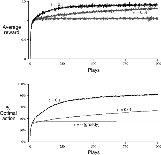
The author explains in 2.2 Action-Value Methods:

To roughly assess the relative effectiveness of the greedy and $\varepsilon $-greedy methods, we compared them numerically on a suite of test problems. This is a set of 2000 randomly generated n-armed bandit tasks with n = 10. For each action, a, the rewards were selected from a normal (Gaussian) probability distribution with mean Q*(a) and variance 1. The 2000 n-armed bandit tasks were generated by reselecting the Q*(a) 2000 times, each according to a normal distribution with mean 0 and variance 1. Averaging over tasks, we can plot the performance and behavior of various methods as they improve with experience over 1000 plays, as in Figure 2.1. We call this suite of test tasks the 10-armed testbed.

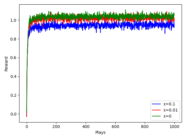
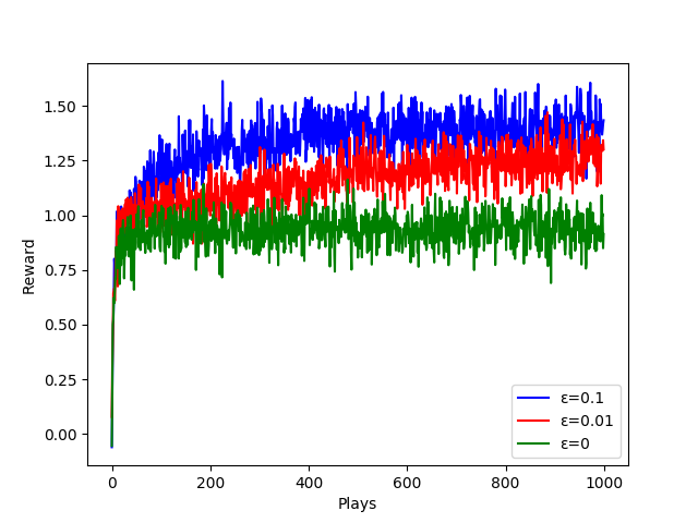
But doing my best, the replication yields something nearer to :

I think I am misunderstanding how the author took the averages.

Here is my code:

from math import exp

import numpy
import matplotlib.pyplot as plt


def act(action, Qstar):
    return numpy.random.normal(Qstar[action], 1)


def run(epsilon):
    history = [0 for i in range(1000)]

    for task in range(1, 2000):
        Qstar = [numpy.random.normal(0, 1) for i in range(10)]
        Q = [0 for i in range(10)]
        for t in range(1, 1001):
            if numpy.random.randint(0, 100) < epsilon:
                action = numpy.random.randint(0, len(Q))
            elif t == 0:
                action = 0
            else:
                averages = [q/t for q in Q]
                action = averages.index(max(averages))

            reward = act(action, Qstar)
            Q[action] += reward

            history[t-1] += reward

    return [elem/2000 for elem in history]


if __name__ == '__main__':
    plt.plot(run(10), 'b', label="ɛ=0.1")
    plt.plot(run(1), 'r', label="ɛ=0.01")
    plt.plot(run(0), 'g', label="ɛ=0")
    plt.xlabel('Plays')
    plt.ylabel('Reward')
    plt.legend()
    plt.show()

Answer 1

You are calculating the average reward for each action (i.e. bandit arm) incorrectly. You cannot calculate this simply with a list comprehension, and you need to keep a second list storing the number of times each action was taken.

The correct calculation is to divide the total reward obtained from each action by the number of times that action was taken. You are dividing all actions by the total number of actions taken. Adding:

...
counts = [0 for i in range(10)]
...
else:
    averages = []
    for i in range(0, 10):
        averages.append(Q[i]/counts[i] if counts[i] > 0 else 0)
    ...
...
counts[action] += 1

results in working code, and I can generate this graph using 200 samples per method, which looks like a noisier version of the one in the figure you referenced: