Regression using neural network

Question

I'd like to ask for any kind of assistance regarding the following problem:

I was given the following training data: 100 numbers, each one is a parameter, they together define a number X(also given).This is one instance,I have 20 000 instances for training.Next, I have 5000 lines given, each containing the 100 numbers as parameters.My task is to predict the number X for these 5000 instances.

I am stuck because I only know of the sigmoid activation function so far, and I assume it's not suitable for cases like this where the output values aren't either 0 or 1.

So my question is this : What's a good choice for an activation function and how does one go about implementing a neural network for a problem such as this?

Answer 1

Lets mock some data up.

"100 numbers, each one is a parameter, they together define a number X(also given)"

# i.e. size of X_train -> [n x d]
# i.e. size of X_train -> [??? x 100]  , when d = 100

# "I have 20000 instances for training"
# i.e. size of X_train -> [20000 x 100], when n = 20000

import torch
import numpy as np

X_train = torch.rand((20000, 100))
X_train = np.random.rand(20000, 100) # Or using numpy

But what is your Y?

# Since the definition of a regression task, 
# loosely means to predict an output real number
# given an input of d dimension

# So the appropriate Y_train would 
# be of dimension [n x 1] 
# and look like this:

y_train = torch.rand((20000, 1))

y_train = np.random.rand(20000, 1) # Or using numpy

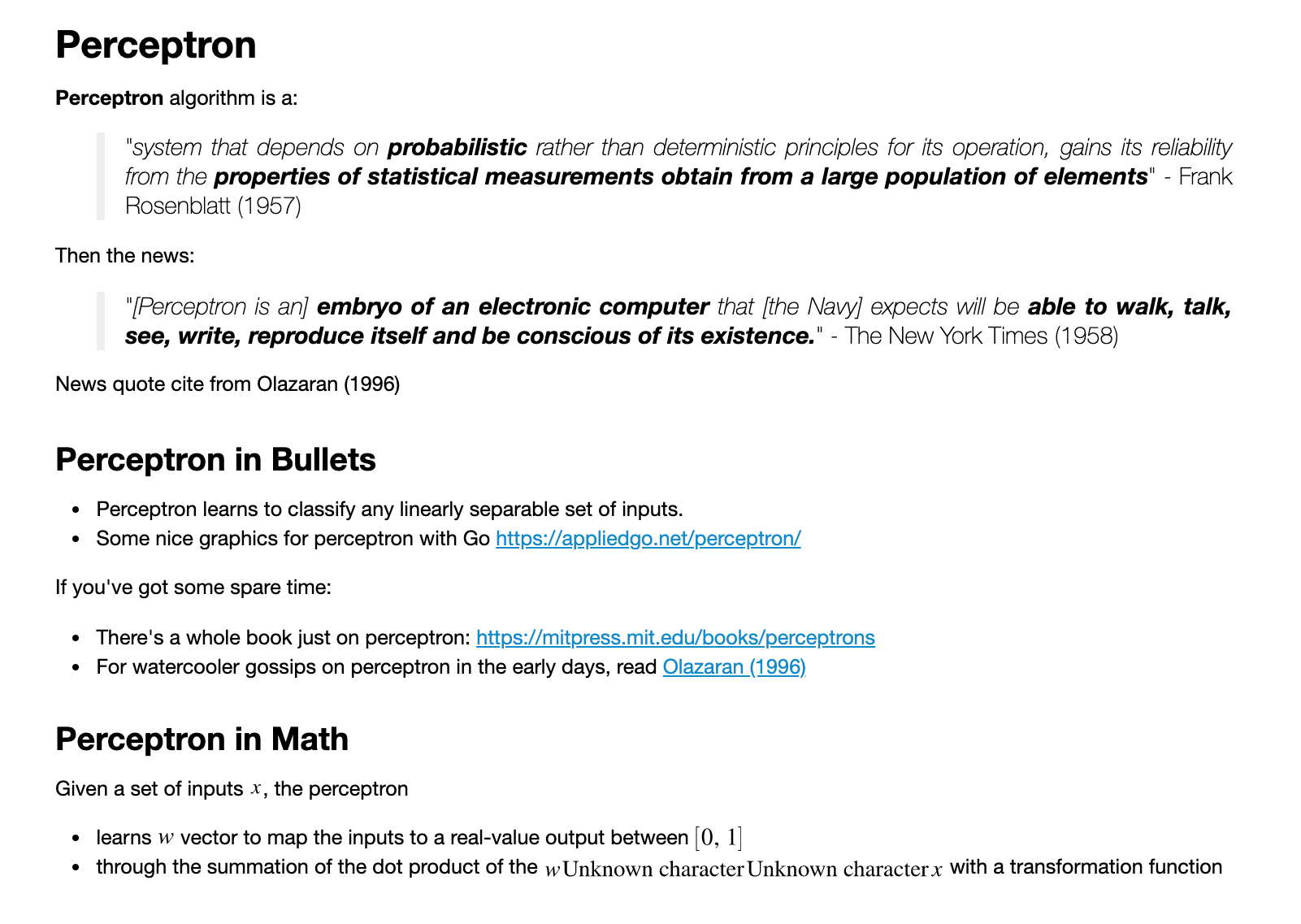
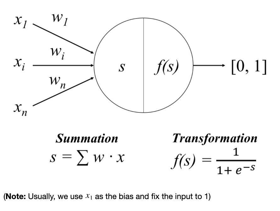
What is a linear perceptron?

Taking definition from this tutorial

Thus, in picture:

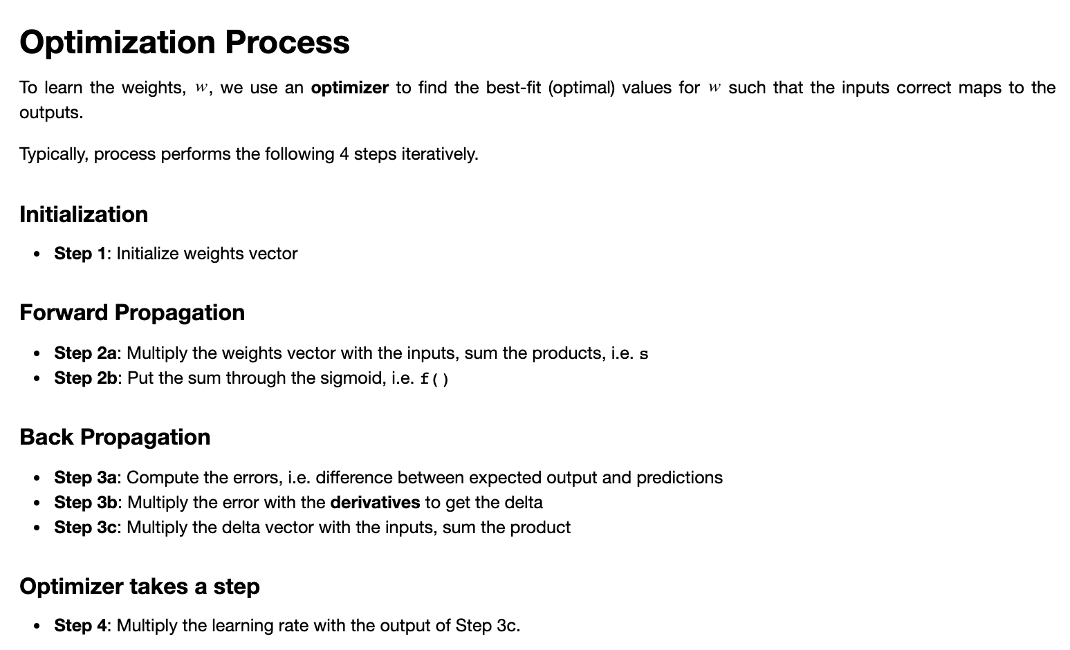
Next we need to define training routine,

For now take it as biblical truth that this is an okay routine to train a neural net model (this isn't the only way but easiest or supervised learning):

In code:

import math
import numpy as np
np.random.seed(0)

def sigmoid(x): # Returns values that sums to one.
    return 1 / (1 + np.exp(-x))

def sigmoid_derivative(sx): 
    # See https://math.stackexchange.com/a/1225116
    # Hint: let sx = sigmoid(x)
    return sx * (1 - sx)

def cost(predicted, truth):
    return np.abs(truth - predicted)


num_epochs = 10000 # No. of times to iterate.
learning_rate = 0.03 # How large a step to take per iteration.

# Lets standardize and call our inputs X and outputs Y
X = np.array(torch.rand((20000, 100)))
Y = or_output

for _ in range(num_epochs):
    layer0 = X

    # Step 2a: Multiply the weights vector with the inputs, sum the products, i.e. s
    # Step 2b: Put the sum through the sigmoid, i.e. f()
    # Inside the perceptron, Step 2. 
    layer1 = sigmoid(np.dot(X, W))

    # Back propagation.
    # Step 3a: Compute the errors, i.e. difference between expected output and predictions
    # How much did we miss?
    layer1_error = cost(layer1, Y)

    # Step 3b: Multiply the error with the derivatives to get the delta
    # multiply how much we missed by the slope of the sigmoid at the values in layer1
    layer1_delta = layer1_error * sigmoid_derivative(layer1)

    # Step 3c: Multiply the delta vector with the inputs, sum the product (use np.dot)
    # Step 4: Multiply the learning rate with the output of Step 3c.
    W +=  learning_rate * np.dot(layer0.T, layer1_delta)

Now that we learn the model, i.e. the W.

When we see the data points that we need to use the model on, we apply the same forward propagation step, i.e. layer1 = sigmoid(np.dot(X, W))

Since we have:

I have 5000 lines given, each containing the 100 numbers as parameters.My task is to predict the number X for these 5000 instances.

And in code:

# If we mock up the data,
# it should be the same internal dimension. 
X_test = np.random.rand(5000, 100)

# The desired output just needs to pass through the W and the activation:
# the shape of `output` -> [5000 x 1] , 
# where there's 1 output value for each input.
output = sigmoid(np.dot(X_test, W))

Answer 2

The quick answer is that you want to use an activation function on the output layer that does not compress values to $(0,1)$. Depending on your software, this might be called "linear" or "identity". It looks like Keras just wants you to leave off the activation function: model.add(Dense(1)).

The typical way of thinking of a neural network as a classifier (let's say a binary classifier) is just extending a logistic regression. In fact, when you use a sigmoid activation function on the output node, you're (sort of) running logistic regression on the final hidden layer.

A logistic regression is one type of generalized linear model. The gist of GLM is that some transformation of the the value of interest is a linear function of the feature space.

Let $X$ be the data matrix for the feature space. Let $\beta$ be a parameter vector. Then $\hat{y} = \mathbb{E}[y] = X\beta$ is the linear model, and $g(\mathbb{E}[y]) = X\beta$ is the generalized linear model (vectorized, so apply $g$ to each $y_i$).

But we could extend this to a nonlinear transformation, and when a neural network is a binary classifier, this is precisely what we're doing. Instead of the transformation of $X$ being given by $\beta$ and thus linear, we apply some nonlinear transformation $f$ and get $g(\mathbb{E}[y]) = f(X)$.

The terminology in GLM is "link function", but that is essentially the activation function on the final node(s) of the neural network. Consequently, all of the GLM link functions are in play, and one of those link functions is the identity function. For a GLM, that's just linear regression. For your neural network, it will be a neural network (nonlinear) regression, which sounds like what you want.

Answer 3

Usually you're normalizing the data first, meaning that your whole dataset will be in between 0 and 1. Afterwords after you're having the model predictions, when computing the cost function or evaluating the model, you can apply the inverse of the normalization function.

Answer 4

for regression, you can use a hidden layer with sigmoid, then a LINEAR output layer, where the weighted sum goes straight through, without modification.

this way your output is not restricted to 0-1