Fully convolution networks

A fully convolution network (FCN) is a neural network that only performs convolution (and subsampling or upsampling) operations.

Convolution neural networks

The typical convolution neural network (CNN) is not fully convolutional because it often contains fully connected layers too (which do not perform the convolution operation), which are parameter-rich, in the sense that they have many parameters (compared to their equivalent convolution layers), although the fully connected layers can also be viewed as convolutions with kernels that cover the entire input regions, which is the main idea behind converting a CNN to an FCN.

An example of an FCN

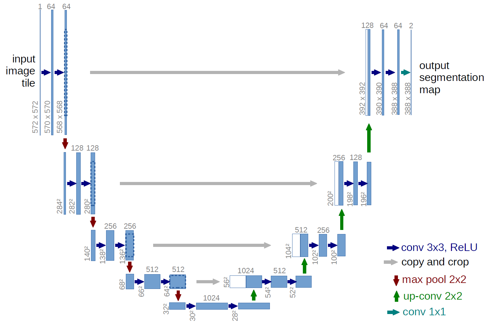
An example of a fully convolutional network is the U-net (called in this way because of its U shape, which you can see from the illustration below), which is a famous network that is used for semantic segmentation, i.e. classify pixels of an image so that pixels that belong to the same class (e.g. a person) are associated with the same label (i.e. person), aka pixel-wise (or dense) classification.

Semantic segmentation

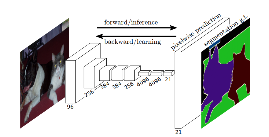
So, in semantic segmentation, you want to associate a label with each pixel (or small patch of pixels) of the input image. Here's an illustration of a neural network that performs semantic segmentation.

Instance segmentation

There's also instance segmentation, where you also want to differentiate different instances of the same class (e.g. you want to distinguish two people in the same image by labeling them differently). An example of a neural network that is used for instance segmentation is mask R-CNN. The blog post Segmentation: U-Net, Mask R-CNN, and Medical Applications (2020) by Rachel Draelos describes these two problems and networks very well.

Here's an example of an image where instances of the same class (i.e. person) have been labeled differently (orange and blue).

Both semantic and instance segmentations are dense classification tasks, that is, you want to classify each pixel or many small patches of pixels of an image.

$1 \times 1$ convolutions

In the U-net diagram above, you can see that there are only convolutions, copy and crop, max-pooling, and upsampling operations. There are no fully connected layers.

So, how do we associate a label to each pixel (or a small patch of pixels) of the input? How do we perform the classification of each pixel (or patch) without a final fully connected layer?

That's where the $1 \times 1$ convolution and upsampling operations are useful!

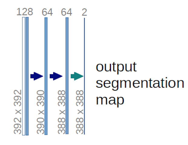
In the case of the U-net diagram above (specifically, the top-right part of the diagram, which is illustrated below for clarity), two $1 \times 1 \times 64$ kernels are applied to the input to produce two feature maps of size $388 \times 388$. They used two $1 \times 1$ kernels because there were two classes in their experiments (cell and not-cell). If you read the mentioned blog post, you will understand this detail.

If you have tried to analyze the U-net diagram carefully, you will notice that the output maps have different spatial (height and weight) dimensions than the input images, which have dimensions $572 \times 572 \times 1$.

That's fine because our general goal is to perform dense classification (i.e. classify patches of the image, where the patches can contain only one pixel), although I said that we would have performed pixel-wise classification, so maybe you were expecting the outputs to have the same exact spatial dimensions of the inputs. However, note that, in practice, you could also have the output maps to have the same spatial dimension as the inputs: you would just need to perform a different upsampling (deconvolution) operation.

How $1\times 1$ convolutions work?

A $1 \times 1$ convolution is just the typical 2d convolution but with a $1\times1$ kernel.

As you probably already know (and if you didn't know this, now you know it), if you have a $g \times g$ kernel that is applied to an input of size $h \times w \times d$, where $d$ is the depth of the input volume (which, for example, in the case of grayscale images, it is $1$), the kernel actually has the shape $g \times g \times d$, i.e. the third dimension of the kernel is equal to the third dimension of the input that it is applied to. This is always the case, except for 3d convolutions, but we are now talking about the typical 2d convolutions! See this answer for more info.

So, in the case we want to apply a $1\times 1$ convolution to an input of shape $388 \times 388 \times 64$, where $64$ is the depth of the input, then the actual $1\times 1$ kernels that we will need to use have shape $1\times 1 \times 64$ (as I said above for the U-net). The way you reduce the depth of the input with $1\times 1$ is determined by the number of $1\times 1$ kernels that you want to use. This is exactly the same thing as for any 2d convolution operation with different kernels (e.g. $3 \times 3$).

In the case of the U-net, the spatial dimensions of the input are reduced in the same way that the spatial dimensions of any input to a CNN are reduced (i.e. 2d convolution followed by downsampling operations). The main difference (apart from not using fully connected layers) between the U-net and other CNNs is that the U-net performs upsampling operations, so it can be viewed as an encoder (left part) followed by a decoder (right part).