Introduction
Bag-of-features (BoF) (also known as bag-of-visual-words) is a method to represent the features of images. BoF is inspired by the bag-of-words model often used in the context of NLP, hence the name. In the context of computer vision, BoF can be used for different purposes, such as content-based image retrieval (CBIR), i.e. find an image in a database that is closest to a query image.
Steps
The BoF can be divided into different phases (or steps). To understand all the phases, consider a training dataset $D = \{x_1, \dots, x_N \}$ of $N$ training images. Then BoF proceeds as follows.
- Extract all the raw features (i.e. keypoints and descriptors) from all images in the training dataset $D$. This can be done with SIFT, where each descriptor is a $128$-dimensional vector that represents the neighbourhood of the pixels around a certain keypoint (e.g. a pixel that represents a corner of an object in the image). For more details about this extraction of features, you should read the SIFT paper.
Note that image $x_i \in D$ may contain a different number of features (keypoints and descriptors) than image $x_j \neq x_i \in D$. As we will see in the next step, BoF produces a feature vector of size $k$ for all images, so all images will be represented by a fixed-size vector.
Let $F= \{f_1, \dots, f_M\}$ be the set of descriptors extracted from all training images in $D$, where $M \gg N$. So, $f_i$ may be a descriptor that belongs to any of the training examples (it does not matter to which training image it belongs, in this phase).
- Cluster all descriptors $F= \{f_1, \dots, f_M\}$ into $k$ clusters using k-means (or another clustering algorithm). This is sometimes known as the vector quantization (VQ) step. In fact, the idea behind VQ is very similar to clustering and sometimes VQ is used interchangeably with clustering.
So, after this phase, we will have $k$ clusters, each of them associated with a centroid $C = \{ c_1, \dots, c_k\}$, where $C$ is the set of centroids (and $c_i \in \mathbb{R}^{128}$ in the case that SIFT descriptors have been used). These centroids represent the main features that are present in the whole training dataset $D$. In this context, they are often known as the codewords (which derives from the vector quantization literature) or visual words (hence the name bag-of-visual-words). The set of codewords is often called codebook or, equivalently, the visual vocabulary.
Now, for simplicity, let's assume that we want to perform CBIR. Given a new image $u \not\in D$ (often called the query image, in this context), then, first, we will represent $u$ as a $k$-dimensional vector (where $k$, if you remember, is the number of codewords). To do that, we need to follow the following steps.
Extract the raw features from $u$ with e.g. SIFT (as we did for the training images). Let the descriptors of $u$ be $U = \{ u_1, \dots, u_{|U|} \}$.
Create a vector $I \in \mathbb{R}^k$ of size $k$ filled with zeros, where the $i$th element of $I$ corresponds to the $i$th codeword (or cluster).
For each $u_i \in U$, find the closest codeword (or centroid) in $C$. Once you found it, increment the value at the $j$th position of $I$ (i.e., initially, from zero to $1$), where $j$ is the closest codeword to the descriptor $u_i$ of the query image.
The distance between $u_i$ and any of the codewords can be computed e.g. with the Euclidean distance. Note that the descriptors of $u$ and the codewords have the same dimension because they have been computed with the same feature descriptor (e.g. SIFT).
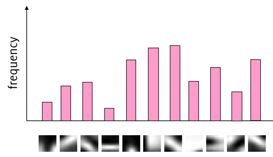
At the end of this process, we will have a vector $I \in \mathbb{R}^k$ that represents the frequency of the codewords in the query image $u$ (akin to the term frequency in the context of the bag-of-words model). $I$ represents a histogram of features of the query image $u$, i.e. the feature vector of $u$. Here's an illustrative example of such a histogram.
From this diagram, we can see that there are $11$ codewords (of course, this is an unrealistic scenario!), and, on the y-axis, we have the frequency of each of the codewords in a given image.
Alternatively, rather than the codeword frequency, we can use the tf-idf. In that case, each image will be represented not by a vector that contains the frequency of the codewords but it will contain the frequency of the codewords weighted by their presence in other images. See this paper for more details (where they show how to calculate tf-idf in this context; specifically, section 4.1, p. 8 of the paper).
To conclude, BoF is a method to represent features of an image, which could then be used to train classifiers or generative models to solve different computer vision tasks (such as CBIR). The first two steps above are concerned with the creation of a visual vocabulary (or codebook), which is then used to create the feature vector of a new test (or query) image.
Further reading
For more info, I suggest that you read the following papers
- Video Google: A Text Retrieval Approach to Object Matching in Videos (2003) by Sivic and Zisserman
- A Bayesian Hierarchical Model for Learning Natural Scene Categories (2005) by Fei-Fei and Perona
- Introduction to the Bag of Features Paradigm for Image Classification and Retrieval (2011) by O'Hara and Draper
- Bag-of-Words Representation in Image Annotation: A Review (2012) by Tsai

