In $Q$-learning there is what is known as a maximisation bias. That is because the update target is $r + \gamma \max_a Q(s,a)$. If you slightly overestimate your $Q$-value then this error gets compounded (there is a nice example in the Sutton and Barto book that illustrates this). The idea behind tabular double $Q$-learning is to have two $Q$-networks, $Q_1,Q_2$, and you choose an action $a$ from them, e.g. from $Q_1 + Q_2$. You then flip a coin to decide which to update. If you choose to update $Q_1$ then the update target becomes $r + \gamma Q_2(s', \arg\max_a Q_1(s',a))$.
The idea is that if you overshoot your estimate on one $Q$ network then having the second will hopefully control this bias when you would take the max.
In Deep Double $Q$-learning the idea is essentially the same but instead of having to maintain and train two $Q$-networks, they use the target network from vanilla DQN to provide the target. To make this more concrete, the update target they use is
$$r + \gamma Q(s', \arg\max_aQ(s',a;\theta);\theta^-)\;,$$
where $Q(s,a;\theta^-)$ denotes the target network whose parameters are only updated to the current networks every $C$ time steps.
As before, the idea is that if we have overestimated our value of being state $s'$ in our current network when taking the max action, using the target network to provide the target will help control for this bias.
Maximisation Bias
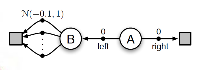
I will here explain maximisation bias from the simple example given from the Sutton and Barto book.

The Markov Decision Process in the image is defined as follows: we start in state A and can take the 'right' action which gives us 0 reward and immediately leads to termination. If we choose 'left' we get 0 immediate reward where we then move to state B. From there, we have an arbitrary number of action we can take where they all lead to the terminal state and the reward is drawn from a Normal(-0.1,1) distribution.
Clearly, the optimal action is always to move to the right from state A as this gives 0 expected future returns. Taking the left action will give a $\gamma \times -0.1$ expected future returns (the $\gamma$ is our discount factor).
Now, if we got into state $B$ and took some random action our initial reward could be bigger than 0 -- after all it is drawn from a Normal(-0.1,1) distribution.
Now, consider we are updating our $Q$-function for state A and taking the left action. Our update target will be $0 + \gamma \max_a Q(B,a)$. Because we are taking the max over all possible actions, this will lead to a positive reward and so we are backing up the belief of our expected future rewards from taking action left in state A to be something positive -- clearly this is wrong since we know it should be -0.1. This is what is known as the maximisation bias, because it gives us a kind of 'optimistic' estimate of the action value!
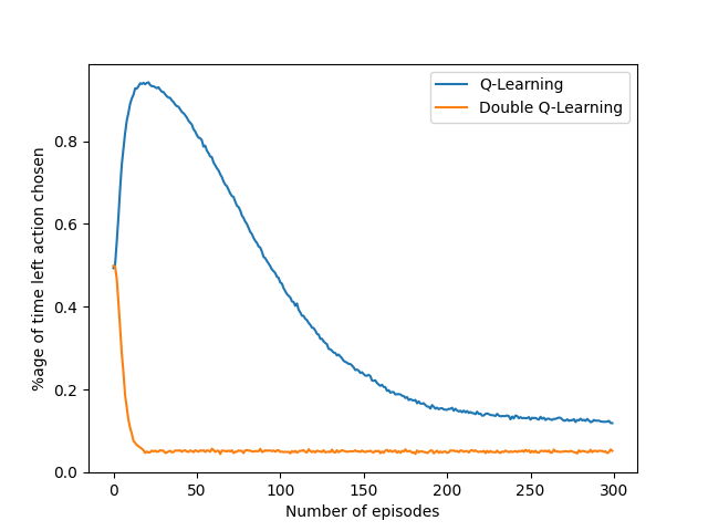
I've attached an image below that shows the %age of time the agent chose the left action, which it shouldn't be choosing). As you can see, it takes normal $Q$-learning along time to even start to correct itself, whereas double $Q$-learning corrects the mistake almost immediately.


