In online one step actor critic, why does the weights update become less significant as the episode progresses?

Question

The Reinforcement Learning Book by Richard Sutton et al, section 13.5 shows an online actor critic algorithm.

Why do the weights updates depend on the discount factor via $I$?

It seems that the more we get closer to the end of the episode, the less we value our newest experience $\delta$.

This seems odd to me. I thought discounting in the recursive formula of $\delta$ itself is enough.

Why does the weights update become less significant as the episode progresses? Note this is not eligibility traces, as those are discussed separately, later in the same episode.

Answer 1

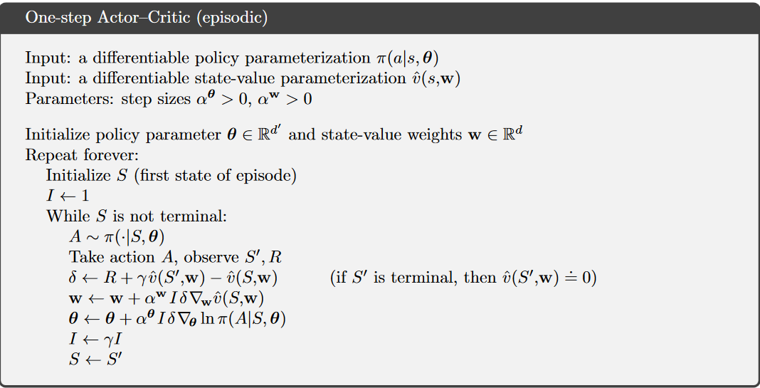
This "decay" of later values is a direct consequence of the episodic formula for the objective function for REINFORCE:

$$J(\theta) = v_{\pi_\theta}(s_0)$$

That is, the expected return from the first state of the episode. This is equation 13.4 in the book edition that you linked in the question.

In other words, if there is any discounting, we care less about rewards seen later in the episode. We mainly care about how well the agent will do from its starting position.

This is not true for all formulations of policy gradients. There are other, related, choices of objective function. We can formulate the objective function as caring about the returns from any distribution of states, but in order to define it well, we do need to describe the weighting/distribution somehow, it should be relevant to the problem, and we want to be able to get approximate samples of $\nabla J(\theta)$ for policy gradient to work. The algorithm you are asking about is specifically for improving policy for episodic problems. Note you can set $\gamma = 1$ for these problems, so the decay is not necessarily required.

As an aside (because someone is bound to ask): Defining $J(\theta)$ with respect to all states equally weighted could lead to difficulties e.g. the objective would take less account of a policy's ability to avoid undesirable states, and it would require a lot of samples from probably irrelevant states in order to estimate it. These difficulties would turn up as a hard to calculate (or maybe impossible) expectation for $\nabla J(\theta)$