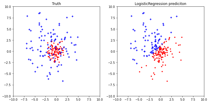
The paper has sources, that contains these plots in pdf. I've converted those to svg and managed to rip the actual data:
xdata = [-0.6,-3.33,-1.93,0.67,-2.63,-3.1,-5.93,-1.87,-3.93,-3.47,1.0,-3.43,-3.83,0.6,-0.47,-3.6,-1.37,-4.87,-3.63,3.53,4.33,1.73,2.63,4.13,-0.13,2.33,-1.6,-6.83,-1.5,-6.37,3.73,0.2,-0.73,-3.17,2.43,-0.3,-1.2,-1.97,-0.3,-2.9,-2.13,-1.4,4.67,0.5,1.13,-6.7,1.1,1.97,0.73,-1.27,4.9,-1.7,-2.3,-5.83,-4.27,-3.93,-5.67,-6.83,-3.7,-0.73,-3.5,-3.63,-6.0,1.5,-1.23,2.23,0.17,-1.43,-0.2,-1.43,1.17,-4.03,2.87,-1.13,-0.7,0.63,-6.27,2.03,-1.23,-2.63,-1.97,-2.3,-1.33,-3.77,-6.07,4.47,0.37,-4.37,3.27,1.3,-5.47,-5.5,2.47,-0.23,-3.97,1.87,-0.37,-3.63,0.77,-3.3,-0.08,-0.95,-0.52,0.32,-0.72,-0.88,-1.78,-0.48,-1.15,-0.98,0.42,-0.98,-1.12,0.28,-0.05,-1.02,-0.32,-1.45,-1.05,1.22,1.48,0.65,0.92,1.42,0.05,0.85,-0.42,-2.05,-0.38,-1.92,1.28,0.15,-0.12,-0.88,0.88,0.02,-0.28,-0.52,0.02,-0.82,-0.58,-0.35,1.58,0.25,0.45,-2.02,0.45,0.72,0.35,-0.28,1.65,-0.42,-0.62,-1.75,-1.25,-1.15,-1.68,-2.05,-1.08,-0.12,-1.02,-1.05,-1.78,0.58,-0.28,0.82,0.15,-0.35,0.05,-0.35,0.48,-1.18,1.02,-0.25,-0.12,0.32,-1.88,0.75,-0.28,-0.72,-0.52,-0.62,-0.32,-1.08,-1.82,1.52,0.22,-1.28,1.15,0.52,-1.62,-1.65,0.88,0.02,-1.15,0.68,-0.02,-1.05,0.35,-0.95]
ydata = [-1.47,-3.18,3.97,5.82,3.47,-1.12,4.58,-6.23,3.03,5.52,-1.07,3.38,8.57,0.43,2.33,4.42,1.12,-4.57,-0.07,1.82,-0.18,0.93,-0.57,1.38,0.57,0.03,-4.82,0.68,-0.97,-1.82,7.82,-3.38,3.78,-1.03,7.52,2.53,3.32,1.43,-2.32,2.42,-5.57,0.53,-1.97,-3.07,-0.28,7.88,-3.07,2.88,1.93,-3.68,3.12,-0.62,7.12,2.22,0.32,6.28,0.78,1.72,-0.07,4.78,2.42,1.12,-1.93,-6.68,3.18,0.53,3.32,-5.18,2.68,-1.93,2.68,8.48,-1.28,2.58,-0.72,6.18,4.82,3.08,2.22,-0.93,0.57,-0.28,4.12,-1.03,0.62,1.43,-4.53,-3.62,3.18,0.53,0.22,-2.72,4.22,1.03,5.88,2.62,3.88,-0.07,-0.47,4.82,-0.88,-1.53,0.82,1.53,0.62,-0.82,0.88,-2.43,0.43,1.28,-0.68,0.57,2.22,-0.22,0.32,0.93,-0.07,-1.97,-0.53,0.32,-0.28,-0.03,-0.47,0.22,-0.18,-0.28,-1.97,-0.38,-0.72,-1.18,2.22,-1.43,0.82,-0.82,2.12,0.43,0.62,0.03,-1.12,0.28,-2.22,-0.28,-0.82,-1.32,-0.43,1.88,-1.32,0.62,0.28,-1.57,0.78,-0.62,1.82,0.12,-0.43,1.47,-0.32,-0.07,-0.53,1.12,0.28,-0.12,-1.18,-2.43,0.57,-0.12,0.68,-2.07,0.47,-1.03,0.53,2.17,-0.68,0.43,-0.62,1.62,0.93,0.68,0.28,-0.78,-0.28,-0.53,0.88,-0.82,-0.38,0.22,-1.82,-1.68,0.72,-0.18,-0.47,-1.43,1.07,-0.07,1.38,0.53,0.88,-0.53,-0.53,1.03]
fake = [1,1,1,1,1,1,1,1,1,1,1,1,1,1,1,1,1,1,1,1,1,1,1,1,1,1,1,1,1,1,1,1,1,1,1,1,1,1,1,1,1,1,1,1,1,1,1,1,1,1,1,1,1,1,1,1,1,1,1,1,1,1,1,1,1,1,1,1,1,1,1,1,1,1,1,1,1,1,1,1,1,1,1,1,1,1,1,1,1,1,1,1,1,1,1,1,1,1,1,1,0,0,0,0,0,0,0,0,0,0,0,0,0,0,0,0,0,0,0,0,0,0,0,0,0,0,0,0,0,0,0,0,0,0,0,0,0,0,0,0,0,0,0,0,0,0,0,0,0,0,0,0,0,0,0,0,0,0,0,0,0,0,0,0,0,0,0,0,0,0,0,0,0,0,0,0,0,0,0,0,0,0,0,0,0,0,0,0,0,0,0,0,0,0,0,0,0,0,0,0]
I feed that into LogisticRegression classifier - which is another way to say that you use a sigmoid for discrimination:
X , y = np.array([xdata,ydata]).T , np.array(fake, dtype=bool)
from sklearn.linear_model import LogisticRegression
lr = LogisticRegression()
lr.fit(X,y)
And I'm plotting the true data on the left and the LogisticRegression on the right:
subplot(121);xlim(-10,10);ylim(-10,10);title("Truth")
scatter(X[~y][:,0], X[~y][:,1],c="r", marker=".")
scatter(X[ y][:,0], X[ y][:,1],c="b", marker="+")
subplot(122);xlim(-10,10);ylim(-10,10);title("LogisticRegression prediciton")
p = lr.predict(X)
scatter(X[~p][:,0], X[~p][:,1],c="r", marker=".")
scatter(X[ p][:,0], X[ p][:,1],c="b", marker="+")
Here you can see the sigmoid decision boundary reproduced.

 .
.
