If $t^i - o^i$ is negative, doesn't the power of 2 eliminate any negative result?
In the loss function, yes that is correct, and is what you want - a measurement that gets higher due to any difference between the predicted and correct results. Minimising the value of that measurement is a goal for the optimiser.
How can then exist any negative gradient at the output?
The gradient of the cost function is different to the cost function. Technically it is the derivative of the cost function with respect to the parameters you can change. Taking the derivative changes the powers in the equation.
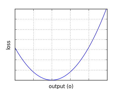
If you plot the graph from a single example, you can clearly see the gradient is negative when the prediction is too low, and positive when the prediction is too high:

Note this is the opposite relationship to the one you suggest in the question. That is why it is called gradient descent when we apply corrections. The steps to correct the parameters are in the opposite direction to the gradient.
In terms of algebra (and moving the example index into a subscript so that is doesn't get in the way visually), assuming $o_i$ is your output value, and $t_i$ is the target value, then you want the gradient of your loss function $L$ with respect to $o_i$ or $\frac{\partial L}{\partial o_i}$:
$$\frac{\partial L}{\partial o_i} = \frac{\partial}{\partial o_i} \frac{1}{2}(t_i - o_i)^2 = \frac{\partial}{\partial o_i} \frac{1}{2}(t_i^2 - 2t_i o_i + o_i^2) = \frac{1}{2}(-2t_i + 2o_i) = o_i - t_i$$
This simple gradient value is negative if your output $o_i$ is lower than the target $t_i$, and positive if $o_i$is greater than $t_i$.
As an aside, if you wondered why the multiplier of $\frac{1}{2}$ was included in the definition of SSE, it is intended by design to end up with this simple result. Without it, everything works, just you would end up with the gradient being $2(o_i - t_i)$

