Based on this repository:
https://github.com/arkm97/svm-from-scratch/blob/master/SVM_from_scratch.ipynb
I will try to reverse engineering that concept:
So firstly there is issue for DataCleaning(removing 0,values, serialize, normalize)
normalizing dataset (replaced by its difference from the mean)
credit_df_norm = (credit_df - credit_df.mean())/(credit_df.std())
Divide dataset into Train & Test:
train_df = credit_df_norm.drop(target, axis=1).loc[:training_points]
train_target = credit_df_norm[target].replace(0, -1).loc[:training_points]
And here is starting the clue of that algorithms (with maths etc.)
given data points $\vec x_j \in \mathbb{R}^{1 \times N}$ and targets
$y_j = \pm 1$, where $j = 1, \dots, M$, find the maximum-margin
hyperplane that separates the two classes ($y_j = 1$ and $y_j = -1$).
Let $\vec w$ be the vector normal to the hyperplane. We want to find
$\vec w$ that satisfies
$$ y_j (\vec w \cdot \vec x_j + b) \geq 1 $$ The dual formulation of
the above is equivalent to maximizing the following over the
multipliers $\vec \alpha$:
$$ L(\vec \alpha) = \vec y \cdot \vec \alpha - \frac 1 2 \vec \alpha
> K \vec \alpha^T$$ subject to the constraints $\sum_{j=1}^M \alpha_j =
> 0$ and $y_j \alpha_j \geq 0$. The matrix $K$ defines the kernel of the
SVM; I've chosen $K_{jk} = k(\vec x_j, \vec x_k) = \vec x_j \cdot \vec
> x_k$. The parameters of the plane are recovered from $\vec w = \vec
> \alpha \cdot \vec x$ and $b = y_j = \vec w \cdot \alpha_j$ for $j$
such that $\alpha_j \neq 0$
Let's divide it to the single factors:
we need to find maximum-margin-hyperplane for separate into two classes:
Separation cause SVN is classification - so we need to classify elements into categories.
𝑦𝑗 = 1
𝑦𝑗 = −1
This pattern allow to find hyperplane(?)
𝑦𝑗(𝑤⃗ ⋅𝑥⃗ 𝑗+𝑏)≥1
The next pattern:
𝐿(𝛼⃗ )=𝑦⃗ ⋅𝛼⃗ −12𝛼⃗ >𝐾𝛼⃗ 𝑇
The author for kernel SVN choose those pattern:
𝐾𝑗𝑘=𝑘(𝑥⃗ 𝑗,𝑥⃗ 𝑘)=𝑥⃗ 𝑗⋅>⃗ 𝑥𝑘
And the parameters for plane are here:
𝑤⃗ =>⃗ 𝛼⋅𝑥⃗ and 𝑏=𝑦𝑗=𝑤⃗ ⋅𝛼𝑗 for 𝑗 such that 𝛼𝑗≠0
Reference:
https://arxiv.org/pdf/1307.0471.pdf
In this line are added the kernel
Popular kernels are:
Polynomial Kernel,
Gaussian Kernel,
Radial Basis Function (RBF),
Laplace RBF Kernel,
Sigmoid Kernel,
Anove RBF Kernel
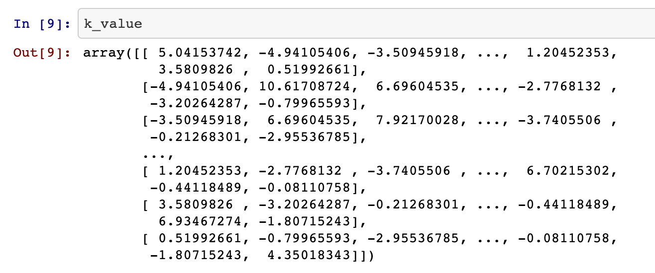
k_value = np.array(train_df @ train_df.T + np.identity(len(train_target))*1e-12)
The structure of k_value (kernel matrix) is an array.

Next there is use of cholesky decomposition—cholesky - which is next complicated concept.
np.linalg.cholesky(k_value)
Next some bits of data converting:
alpha = cp.Variable(shape=train_target.shape)
beta = cp.multiply(alpha, train_target) # to simplify notation
K = cp.Parameter(shape=k_value.shape, PSD=True, value=k_value)

# objective function
obj = .5 * cp.quad_form(beta, K) - np.ones(alpha.shape).T @ alpha

# constraints
const = [np.array(train_target.T) @ alpha == 0,
        -alpha <= np.zeros(alpha.shape),
        alpha <= 10*np.ones(shape=alpha.shape)]
prob = cp.Problem(cp.Minimize(obj), const)
The next step is recreate the hyperplane:
w = np.multiply(train_target, alpha.value).T @ train_df
S = (alpha.value > 1e-4).flatten()
b = train_target[S] - train_df[S] @ w
b = b[0]
# b = np.mean(b)
And finally - the classification and evaluation:
def classify(x):
    result = w @ x + b
    return np.sign(result)

correct = 0
incorrect = 0
validation_set = credit_df_norm.drop(target, axis=1)
predictions = []
for i, x in validation_set.iterrows():
    my_svm = classify(x)
    if my_svm==credit_df_norm[target].replace(0, -1)[i]: correct +=1
    else: incorrect +=1
    predictions.append(my_svm)
predictions = np.array(predictions)


print(f"fraction correct: {correct/(correct + incorrect)}")
That was the more detailed implementation - for shorcut there is an interesting article:
https://towardsdatascience.com/svm-and-kernel-svm-fed02bef1200
There are existing function from another library - that can be reused in simple manner:
# Fitting SVM to the Training set
from sklearn.svm import SVC
classifier = SVC(kernel = 'rbf', C = 0.1, gamma = 0.1)
classifier.fit(X_train, y_train)

%matplotlib inline
import numpy as np
import matplotlib.pyplot as plt
from scipy import stats

# use seaborn plotting defaults
import seaborn as sns; sns.set()
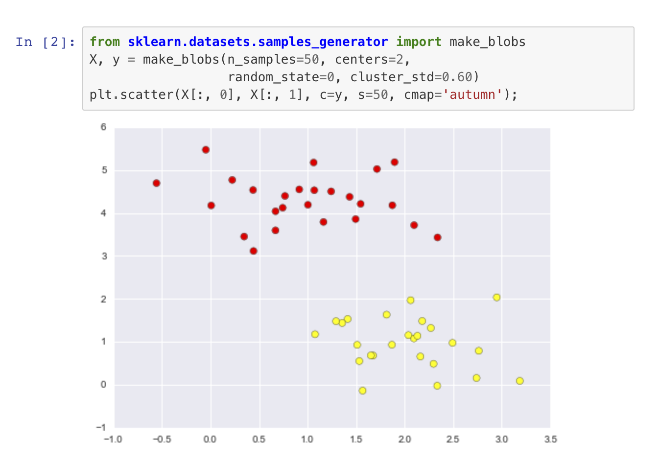
Visualized Dataset:

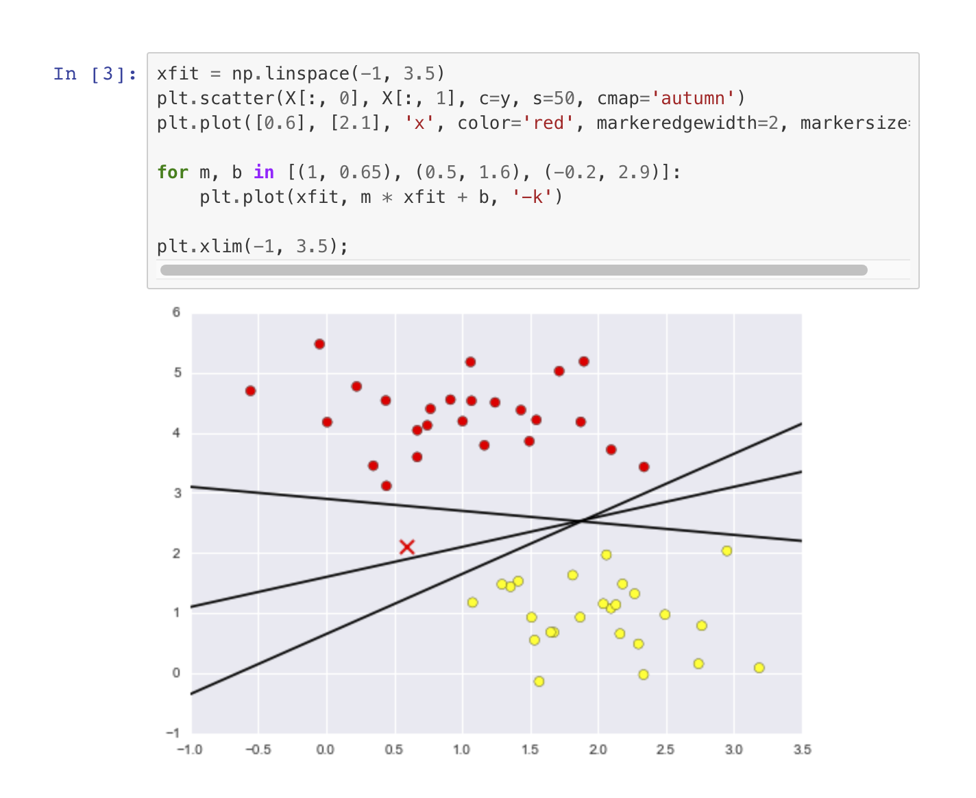
Dataset after apply hyperplanes:
