3
$\begingroup$

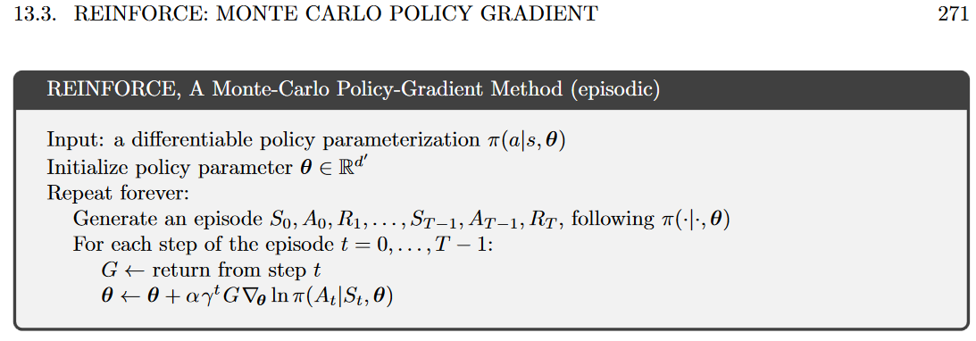
From the reinforcement learning book section 13.3:

enter image description here

Using pytorch, I need to calculate a loss, and then the gradient is calculated internally.

How to obtain the loss from equations which are stated in the form of an iterative update with respect to the gradient?

In this case:

$\theta \leftarrow \theta + \alpha\gamma^tG\nabla_{\theta}ln\pi(A_t|S_t,\theta)$

What would be the loss?

And in general, what would be the loss if the update rule were

$\theta \leftarrow \theta + \alpha C\nabla_{\theta}g(x|\theta)$

for some general (derivable) function $g$ parameterized by theta?

$\endgroup$
6
  • $\begingroup$ Why do you need to calculate any loss here? You need to compute the derivate with respect to $\theta$ of $\ln \pi (A_t \mid S_t, \theta)$. I suppose that $\pi (A_t \mid S_t, \theta)$ will be represented as a neural network. You're not performing supervised learning. $\endgroup$
    – nbro
    Feb 12, 2019 at 13:08
  • $\begingroup$ If I were to implement this with pytorch, I would need to calculate some kind of loss in order to update the policy $\pi$. I simply don't quite understand how to transform the iterative notation to a loss notation (which would then be fed into the optimizer) $\endgroup$
    – Gulzar
    Feb 12, 2019 at 13:17
  • $\begingroup$ Have you had a look at the examples here: github.com/pytorch/examples/tree/master/reinforcement_learning? $\endgroup$
    – nbro
    Feb 12, 2019 at 15:46
  • $\begingroup$ @nbro this is my only question here in which I haven't linked to one of the code examples there :). My question is more general, because I want to go on to the next algorithms in the book, and then onwards for example algorithm 13.5, for which there is no code in the linked pytorch example. $\endgroup$
    – Gulzar
    Feb 12, 2019 at 15:49
  • $\begingroup$ your "loss" would be $-ln(\pi(a\mid s, \theta))G\gamma^t$, I somewhat answered your question here. In this case $A$ that i wrote there would be $G\gamma^t$ $\endgroup$
    – Brale
    Feb 12, 2019 at 16:51

2 Answers 2

3
$\begingroup$

You can find an implementation of the REINFORCE algorithm (as defined in your question) in PyTorch at the following URL: https://github.com/JamesChuanggg/pytorch-REINFORCE/. First of all, I would like to note that a policy can be represented or implemented as a neural network, where the input is the state (you are currently in) and the output is a "probability distribution over the actions you can take from that state received as input".

In the Python module https://github.com/JamesChuanggg/pytorch-REINFORCE/blob/master/reinforce_discrete.py, the policy is defined as a neural network with 2 linear layers, where the first linear layer is followed by a ReLU activation function, whereas the second is followed by a soft-max. In that same Python module, the author also defines another class called REINFORCE, which creates a Policy object (in the __init__ method) and defines it as property of that class. The class REINFORCE also defines two methods select_action and update_parameters. These two methods are called from the main.py module, where the main loop of the REINFORCE algorithm is implemented. In that same main loop, the author declares lists entropies, log_probs and rewards. Note that these lists are re-initialized at ever episode. A "log_prob" and an "entropy" is returned from the select_action method, whereas a "reward" is returned from the environment after having executed one environment step. The environment is provided by the OpenAI's Gym library. The lists entropies, log_probs and rewards are then used to update the parameters, i.e. they are used by the method update_parameters defined in the class REINFORCE.

Let's see better now what these methods, select_action and update_parameters, actually do.

select_action first calls the forward method of the class Policy, which returns the output of the forward pass of the NN (i.e. the output of the soft-max layer), so it returns the probabilities of selecting each of the available actions (from the state given as input). It then selects the probability associated with the first action (I guess, it picks the probabilities associated with the action with the highest probabilities), denoted by prob (in the source code). Essentially, what I've described so far regarding this select_action method is the computation of $\pi(A_t \mid S_t, \theta)$ (as shown in the pseudocode of your question). Afterwards, in the same method select_action, the author also computes the log of that probability I've just mentioned above (i.e. the one associated with the action with the highest probability, i.e. the log of prob), denoted by log_prob. In that same method, the entropy (as defined in this answer) is calculated. In reality, the author calculates the entropy using only one distribution (instead of two): more specifically, the entropy is calculated as follows entropy = -(probs*probs.log()).sum(). In fact, the entropy loss function usually requires the ground-truth labels (as explained in the answer I linked you to above), but, in this case, we do not have ground-truth labels (given that we are performing RL and not supervised learning). Nonetheless, I can't really tell you why the entropy is calculated like this, in this case. Finally, the method select_action then return action[0], log_prob, entropy.

First of all, I would like to note that the method update_parameters is called only at the end of each episode (in the main.py module). In that same method, a variable called loss is first initialized to zero. In that method, we then iterate the list of rewards for the current episode. Inside that loop of the update_parameters method, the return, R is calculated. R is also multiplied by $\gamma$. On each time step, the loss is then calculated as follows

loss = loss - (log_probs[i]*(Variable(R).expand_as(log_probs[i])).cuda()).sum() - (0.0001*entropies[i].cuda()).sum()

The loss is calculated by subtracting the previous loss with

(log_probs[i]*(Variable(R).expand_as(log_probs[i])).cuda()).sum() - (0.0001*entropies[i].cuda()).sum()

where log_probs are the log probabilities calculated in the select_action method. log_probs is the part $\log \pi(A_t \mid S_t, \theta)$ of the update rule of your pseudocode. log_probs are then multiplied by the return R. We then sum the result of this multiplication over all elements of the vector. We then subtract this just obtained result by the entropies multiplied by 0.0001. I can't really tell you why the author decided to implement the loss in this way. I would need to think about it a little more.

The following article may also be useful: https://pytorch.org/docs/stable/distributions.html.

$\endgroup$
5
  • $\begingroup$ Thanks for all the details! However, my question was mostly theoretical. In most papers i've seen, the update rules are formulated like the pseudocode equations I linked in the question. I wanted to know how IN THE GENERAL CASE I would convert such equations to a loss function. Pseudocode would be enough for this purpose. I'm sorry, but I still can't figure out the equation which loss=... came from. $\endgroup$
    – Gulzar
    Feb 14, 2019 at 16:51
  • $\begingroup$ @Gulzar If you have figured out more details behind my explanations and the linked source code, feel free to add them as an answer to your own question! $\endgroup$
    – nbro
    Mar 14, 2019 at 21:18
  • $\begingroup$ Sorry about that, i had to put that project aside for too many weeks and. I hope i will get back to it asap $\endgroup$
    – Gulzar
    Mar 14, 2019 at 22:59
  • $\begingroup$ @nbro the entropy function you describe is the information theory entropy function found here. The entropy function you refer to with two distributions is the Cross-entropy function, which essentially compares how similar two distributions are. The entropy function used here is the average rate at which information is produced by a stochastic source of data. $\endgroup$
    – Hanzy
    Apr 21, 2019 at 1:54
  • $\begingroup$ The only part of the loss function I can’t discern is why the author subtracts (0.0001*entropies[i]) at each step of calculating the loss. $\endgroup$
    – Hanzy
    Apr 21, 2019 at 3:52
0
$\begingroup$

Chiming in because I had the same question and stumbled across your post. It seems like the general version of your question still has not been answered.

In general, a well-formed gradient update rule is all you need to be able to train the network. We are thinking of converting to a "loss function" because that is the typical flow in the structure that pytorch provides for training networks via their autograd framework.

But the pytorch loss function is really just meant to be the last in a list of nested operations over which we are going to compute gradients. So if you already know your gradient update rule, the easiest way to write it down as a pytorch "loss function" is as the integral of your gradient update rule with respect to the network's output -- then pytorch will compute your gradient update rule for you automatically.

So in your example, the loss function would be:

$-\alpha^tG \ln\pi(A_t | S_t, \theta_t)$

as already noted by @Brale and others. The minus sign is there because pytorch optimizers will typically carry out minimization, but your gradient update rule is intended to maximize.

Hopefully this explanation is helpful to others that are still learning pytorch! Also, I would highly recommend that anyone just getting started with pytorch read their latest autograd tutorial here

$\endgroup$

You must log in to answer this question.

Not the answer you're looking for? Browse other questions tagged .